Natural Gradient Shared Control

How can we combine the controls of both user and robot? How can we give more control authority to the user? 

Our motivation comes from vector fields. We can think of the global autonomous robot policy as a vector field over the whole state space. At any state, the robot policy would want to avoid the obstacles but move towards the goal. Therefore, obstacles can be represented as a “source (positive divergence)” and the goals can be though as a “sink (negative divergence)”.  Depending on the objectives that the autonomous policy optimizes, The environment can have multiple sources and states.

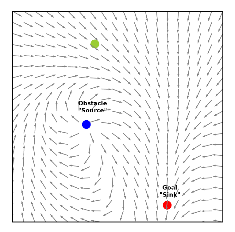
Near these regions (sources & sinks) the autonomous robot can take more control authority to ensure safety or precision. Elsewhere, the user can maintain more control authority in regions where the field does not diverge. We connect this idea with the Fisher information matrix.

We start by formulating shared control as an optimization problem. The shared control action is chosen to maximize the user’s internal action-value function while satisfying a proximity condition that keeps the shared policy close to the autonomous policy. BTW, this is similar to setting a trust region for policy updates in the TRPO reinforcement learning algorithm. 

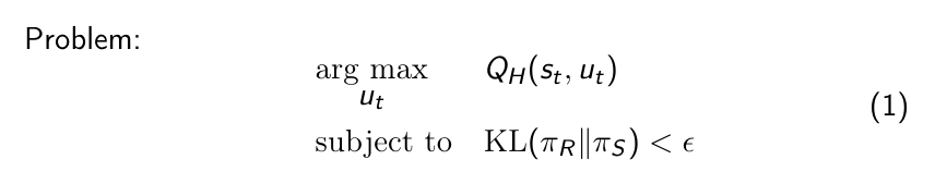
We can solve the problem using a Lagrange Multiplier, by assuming a linear approximation of the objective and quadratic approximation of the KL-divergence. 

This leads to an update rule using natural gradient ascent. Note that our goal is to find the action that maximizes Q_H, resulting in taking gradient steps in the direction of ascent.

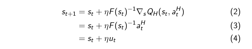
Modeling the user’s internal action-value function Q_H is challenging, so we utilize the user’s action as an estimate of the gradient at each step in Eq. 3.

The Fisher information F, by definition, measures the expectation of the overall sensitivity of a probability distribution p(x|theta) to changes of theta. The Fisher information is the second order derivative of the KL divergence, which is why it emerged from solving Eq. 1. In our settings, the Fisher matrix expresses the sensitivity of the probability distribution p(a|s) to perturbations of the state.

We approximate F as the curvature of the robot’s action-value function at a given state.

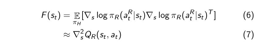
As we consider action as an approximate of the first derivative of the Q function, the Jacobian of the action becomes the Hessian of the Q function.

We represent the autonomous policy as a neural network policy that can be regressed over the whole state space. The network is trained using optimized robot trajectories in a supervised manner.

Thus, to compute the second-order derivative of the Q function, we use the first-order derivative of the actions, using the finite difference method. This can be easily queried using the trained network.

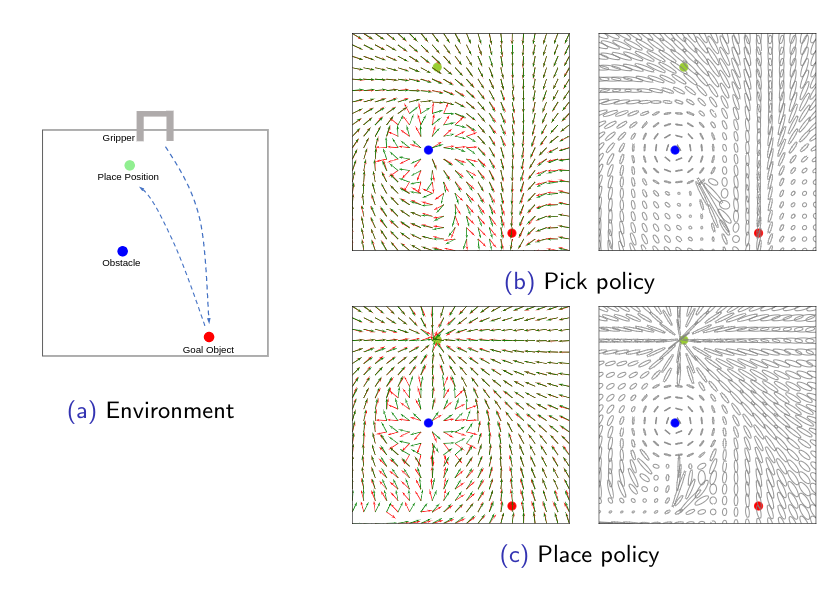
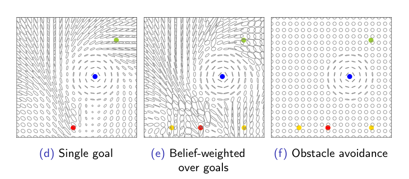
For a pick-and-place task,  we display the ellipses that represent the eigenvalues and the eigenvectors of the inverse Fisher matrix F^(-1). The ellipse represents the direction that the user’s action is stretched along. When the ellipse is close to a circle the user has more control authority over the system. Oppositely, when the ellipse is narrow, for example near an obstacle, the robot augments the user’s actions towards one direction.

We can provide different levels of assistance depending on the cost function that the robot policy optimizes. The robot policy can be either goal directed or it can assist minimally to avoid obstacles. In case of multiple goals, we compute the inverse fisher matrix as a weighted sum over the beliefs. In this case, when the intent is not clear, the robot transfers the control authority to the user.